OpenSees Blog 日本語 目次

最初に「このブログをみるためのガイド」をご覧ください。

Update中OpenSees コマンド 日本語解説 の 目次 OpenSeesコマンド はじめての方は「ここから
このblogで使用しているOpenSeesコマンド集は「ここ」 Update中
OpenSees のソースコード 解析に挑戦してみる 目次最初のページは「ソースコードのダウンロードとビルド」
Appendix:C言語での 「有限要素法における平面トラスの解析」目次最初のページは「Microsoft Visual Studioの導入方法」


目次の中で、更新したページにはNewがついています

このブログ内の単語を検索したい場合は、左上OpenSeesロゴの上に検索窓から検索できます。


2023年4月21日金曜日

2018年4月18日水曜日

Kindle 本 Version 1.1  出しました


日本版


US版  Written in Japanese

修正/追加点は、以下の通りです
V1.0 でありました単位の間違いの修正
PowerShellでOpenSeesを実行する方法
   Microsoft: 最新のWindows 10リリースで「コマンドプロンプト」を削除する方向もある、ということですので、DOSコマンドプロンプトの代わりに、PowerShellでOpenSeesを実行する方法を記載

よろしくお願いします!

2017年11月16日木曜日

OpenSees Basic Examples ( D5: 2階建て単スパンフレームでの固有値解析) 解析結果

2階建て単スパンフレームでの固有値解析(ここ)で作成した、EigenAnal_twoStoreyFrame1.tclファイル内の OpenSeesコマンドを実行すると、以下の様な画面が表示されます。


1次の固有周期は 0.6285387528267521
2次の固有周期は 0.23593885745804652

このデータは、modesフォルダーの中のPeriods.txtの中にもあります

1次の固有振動モード(固有ベクトル)eigenvector は {0.3869004256389495 1.0}
2次の固有振動モード(固有ベクトル)eigenvector は {-1.2923221761110006 1.0}


また、
1次モード、2次モードのx,yの1次、2次の振動モード形を
OpenSeesによりプロットした結果は以下の様になります。

このグラフのデータは、modesフォルダーの中のmode1.outとmode2.outにあります。

Node1 Node2
x y θ x y θ
mode1 0 0 0 0 0 0
mode2 0 0 0 0 0 0

Node3 Node4
x y θ x y θ
mode1 0.666844 0.00224274 -0.00599676 0.666844 #VALUE! -0.00599676
mode2 1.21874 -0.00138942 -0.00256026 1.21874 0.00138942 -0.00256026

Node5 Node6
x y θ x y θ
mode1 1.72355 0.00297706 -0.0058452 1.72355 -0.00297706 -0.0058452
mode2 -0.94306 -0.00342779 0.0161851 -0.94306 0.00342779 0.0161851


Opensees コマンド 日本語解説 : 目次


2017年2月6日月曜日

OpenSees Basic Examples ( D4: 2階建て単スパンフレームでの固有値解析) コマンドサマリ


Basic Examples ( 2階建て単スパンフレームでの固有値解析)   解説
のコマンドのサマリは以下の通りです。

このコマンドを ファイル名 EigenAnal_twoStoreyFrame1.tcl として、テキストフォーマットで作成し、
OpenSeesの起動環境 で 起動しているOpenSees のコマンドラインに

OpenSees EigenAnal_twoStoreyFrame1.tcl  <Enter>

と打ち込んで、実行します。

-----EigenAnal_twoStoreyFrame1.tcl 始まり ------

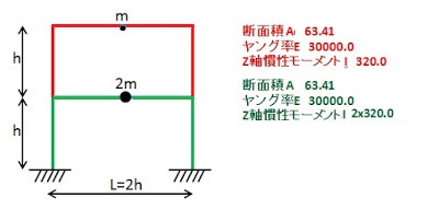
# Eigen analysis of a two-storey one-bay frame; Example 10.5 from "Dynamics of Structures" book by Anil Chopra

# units: kips, in, sec

#       Vesna Terzic, 2010

#delete all previosly constructed objects
wipe;    

#set input variables
#--------------------

#mass
set m  [expr 100.0/386.0]

#number of modes
set numModes 2

#material
set A 63.41
set I 320.0
set E 29000.0

#geometry
set L 240.
set h  120.

# create data directory
file mkdir modes;

# define the model
#---------------------------------
#model builder
model BasicBuilder -ndm 2 -ndf 3

# nodal coordinates:
node 1   0.  0. ;
node 2   $L  0. ;
node 3   0.  $h ;
node 4   $L  $h ;
node 5   0.  [expr 2*$h];
node 6   $L  [expr 2*$h];

# Single point constraints -- Boundary Conditions
fix 1 1 1 1;
fix 2 1 1 1;

# assign mass
mass 3 $m 0. 0. ;
mass 4 $m 0. 0. ;
mass 5 [expr $m/2.] 0. 0. ;
mass 6 [expr $m/2.] 0. 0. ;

# define geometric transformation:
set TransfTag 1;
geomTransf Linear $TransfTag ;

# define elements:
# columns
element elasticBeamColumn 1 1 3 $A $E [expr 2.*$I] $TransfTag;
element elasticBeamColumn 2 3 5 $A $E $I           $TransfTag;
element elasticBeamColumn 3 2 4 $A $E [expr 2.*$I] $TransfTag;
element elasticBeamColumn 4 4 6 $A $E $I           $TransfTag;
# beams
element elasticBeamColumn 5 3 4 $A $E [expr 2.*$I] $TransfTag;
element elasticBeamColumn 6 5 6 $A $E $I           $TransfTag;

# record eigenvectors
#----------------------
for { set k 1 } { $k <= $numModes } { incr k } {
    recorder Node -file [format "modes/mode%i.out" $k] -nodeRange 1 6 -dof 1 2 3  "eigen $k"
}

# perform eigen analysis
#-----------------------------
set lambda [eigen  $numModes];

# calculate frequencies and periods of the structure
#---------------------------------------------------
set omega {}
set f {}
set T {}
set pi 3.141593

foreach lam $lambda {
lappend omega [expr sqrt($lam)]
lappend f [expr sqrt($lam)/(2*$pi)]
lappend T [expr (2*$pi)/sqrt($lam)]
}

puts "periods are $T"

# write the output file cosisting of periods
#--------------------------------------------
set period "modes/Periods.txt"
set Periods [open $period "w"]
foreach t $T {
puts $Periods " $t"
}
close $Periods

# record the eigenvectors
#------------------------
record

# create display  for mode shapes
#---------------------------------
#                 $windowTitle $xLoc $yLoc $xPixels $yPixels
recorder display "Mode Shape 1"  10    10     500      500     -wipe
prp $h $h 1;                                         # projection reference point (prp); defines the center of projection (viewer eye)
vup  0  1 0;                                         # view-up vector (vup)
vpn  0  0 1;                                         # view-plane normal (vpn)  
viewWindow -200 200 -200 200;                        # coordiantes of the window relative to prp
display -1 5 20;                                     # the 1st arg. is the tag for display mode (ex. -1 is for the first mode shape)
                                                     # the 2nd arg. is magnification factor for nodes, the 3rd arg. is magnif. factor of deformed shape
recorder display "Mode Shape 2" 10 510 500 500 -wipe
prp $h $h 1;
vup  0  1 0;
vpn  0  0 1;
viewWindow -200 200 -200 200
display -2 5 20

# get values of eigenvectors for translational DOFs
#---------------------------------------------------
set f11 [nodeEigenvector 3 1 1]
set f21 [nodeEigenvector 5 1 1]
set f12 [nodeEigenvector 3 2 1]
set f22 [nodeEigenvector 5 2 1]
puts "eigenvector 1: [list [expr {$f11/$f21}] [expr {$f21/$f21}] ]"
puts "eigenvector 2: [list [expr {$f12/$f22}] [expr {$f22/$f22}] ]"

after 10000

----- EigenAnal_twoStoreyFrame1.tcl 終わり ------


次のページ →
OpenSees Basic Examples ( D4: 2階建て単スパンフレームでの固有値解析) 解析結果


Opensees コマンド 日本語解説 : 目次

2017年1月25日水曜日

2017年1月18日水曜日

OpenSees Basic Examples ( D2: 2階建て単スパンフレームでの固有値解析) 解説(Node, Element)


0)必要となる数字をシンボルに代入しておき、実行環境を生成します

#input
set m  [expr 100.0/386.0]
set numModes 2      # 解析する固有値モードの数

#material
set A 63.41    # Element 1,2,3,4,5,6の断面積
set I 320.0       #Element 2,4,6の慣性モーメント
set E 29000.0  # ヤング率

#geometry
set L 240.
set h  120.

# create data directory "mkdir"のディレクトリを生成します
file mkdir modes; 


1)Model, Node(節点), Element(要素)の設定
解析する時の、次元、節点(Node)、要素(Element)の
Opensees のコマンドは、以下の通りです。

1.1) 2次元、自由度3 で、解析するよう設定します
model BasicBuilder [次元数] [自由度数] 

model BasicBuilder -ndm 2 -ndf 3

(参照ページはここ

1.2) Node(節点) の 座標を設定します
Node [ nodeの番号 ] [ x座標] [y座標] -mass [節点質量(自由度の第1成分:u )]
[節点質量(自由度の第2成分:v )] [節点質量(自由度の第3成分:θ )]

$がついた変数は、0)の所で定義したシンボルの数字がはいります。


# nodal coordinates:
node 1   0.  0. ;
node 2   $L  0. ;
node 3   0.  $h ;
node 4   $L  $h ;
node 5   0.  [expr 2*$h];    #  = 2 x h 
node 6   $L  [expr 2*$h];       #  = 2 x h 

1.3) Nodeのどこを固定するかを設定します
ここでは、nodeの1と2を固定します。

fix [ nodeの番号 ] [ uの固定の定義]  [ vの固定の定義]  [ θの固定の定義] 
0: 固定されていない
1: 固定されている


# Single point constraints -- Boundary Conditions
fix 1 1 1 1;
fix 2 1 1 1;


(参照ページはここ

1.4) Nodeの質量の定義

Nodeの質量を指定します。

Node3,4  Node5,6 の水平方向のみの質量が定義されています

mass [ nodeの番号 ] [ uの質量]  [ vの質量]  θ回転慣性質量] 


# assign mass
mass 3 $m 0. 0. ;
mass 4 $m 0. 0. ;
mass 5 [expr $m/2.] 0. 0. ;
mass 6 [expr $m/2.] 0. 0. ;

(参照ページはここ

1.5) 座標変換の定義

geomTransf [座標変換の方法] [座標変換方法のID]


# define geometric transformation:
set TransfTag 1;
geomTransf Linear $TransfTag ;


(参照ページはここ


1.6) Element(要素)を設定します。

Element コマンド の中の elasticBeamColum を使用します。

element elasticBeamColumn [ elementの番号 ] [ 片方のnode番号] [片方のnode番号] [ 断面積] [ヤング率] [Z軸の慣性モーメント] [座標変換方法のID]


# define elements:
# columns
element elasticBeamColumn 1 1 3 $A $E [expr 2.*$I] $TransfTag;
element elasticBeamColumn 2 3 5 $A $E $I           $TransfTag;
element elasticBeamColumn 3 2 4 $A $E [expr 2.*$I] $TransfTag;
element elasticBeamColumn 4 4 6 $A $E $I           $TransfTag;
# beams
element elasticBeamColumn 5 3 4 $A $E [expr 2.*$I] $TransfTag;
element elasticBeamColumn 6 5 6 $A $E $I           $TransfTag;


(参照ページはここ


次のページ →
OpenSees Basic Examples ( D3: 2階建て単スパンフレームでの固有値解析)) 解説(固有値解析)


Opensees コマンド 日本語解説 : 目次

2017年1月12日木曜日

OpenSees Basic Examples ( D1: 2階建て単スパンフレームでの固有値解析) 例題


  Eigen analysis of a two-storey one-bay frame 参照


例題は、下図の通りです。
Chopra教授の "Dynamic of Structures" からの例題です
10章  Free Vibration  part A Natural Vibration Frequencies and modes 10.4章 Orthogonality of modes

柱、桁の軸変形は無視、軸力の影響も無視した、理想的な形状として定義しています
軸と桁の断面積、Z軸慣性モーメント、ヤング率は同じ状態としています。

単位は in, kips です


NodeとElementの場所は、下図のとおりです


h = 120
L = 2h = 240

m = 100.0/386.0 (集中質量)

解析する固有値モードの数 2

次のページ →
OpenSees Basic Examples ( D1: 2階建て単スパンフレームでの固有値解析) 解説(Node, Element)


Opensees コマンド 日本語解説 : 目次